Spectral cytometry measures every fluorophore across many detectors, and unmixing turns those detector signals back into one value per marker. Every later step, from gates and clusters to statistics, inherits the errors of that unmixing. Honeychrome’s unmixing is AutoSpectral, developed by Oliver Burton and colleagues in the Liston-Dooley lab at the University of Cambridge and first written as an R package. Honeychrome runs the whole AutoSpectral workflow without any programming.

Why classical unmixing struggles

Classical unmixing fits each cell with one spectrum per fluorophore, measured from single-stained controls, usually by ordinary least squares. Three things go wrong in real samples:

• The control spectra are imperfect. A gate on the peak channel picks up autofluorescent cells as well as stained ones, and an internal negative rarely has the same autofluorescence as the positive cells. The spectrum that results is partly autofluorescence.
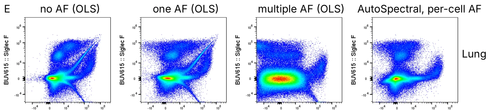
• Autofluorescence varies between cells. It depends on cell type, metabolism and sample preparation, so one autofluorescence spectrum (or none) is wrong for most cells in a tissue. The leftover signal appears as diagonal spikes, skews and false positives.
• Fluorophores vary between cells too. Tandem dyes break down to different degrees and the local environment shifts emission. The spread this causes grows with every similar dye in the panel (Nguyen et al. 2013; Mage et al. 2026).

These artefacts are not built into the instrument. They come from the statistical model used to process the data.

How AutoSpectral works

AutoSpectral extends AutoSpill, our compensation algorithm (Roca et al. 2021), to spectral data. It builds an error-minimised unmixing matrix from cleaned controls, then adds two independent per-cell steps: one for autofluorescence and one for fluorophore variation.

The AutoSpectral pipeline, redrawn from Figure 1 of Burton et al. 2025.

1. Clean spectra from single-stained controls

• Robust linear regression. The signal in each detector is regressed against the fluorophore’s peak detector. Robust regression down-weights events far from the line, so cells whose signal is mostly autofluorescence lose their influence without a hand-drawn gate.
• Scatter matching. The brightest events of each control define its positive population. Unstained cells with the same forward and side scatter are then chosen as its negative, so positives and negatives share an autofluorescence background (Roederer 2002).
• Intrusive autofluorescence removal. Very bright autofluorescent events, such as macrophages and dead cells, are found in the unstained sample and excluded from the control before the spectrum is fitted. Only the controls are filtered; no events are removed from your samples.

Robust regression (right) removes the skew produced by a spectrum from classical positive and negative gates (left). Mouse splenocytes, 42-colour panel. Burton et al. 2025, Figure 3G.

Scatter-matched negatives remove the diagonal error in BV650. Burton et al. 2025, Figure 4E.

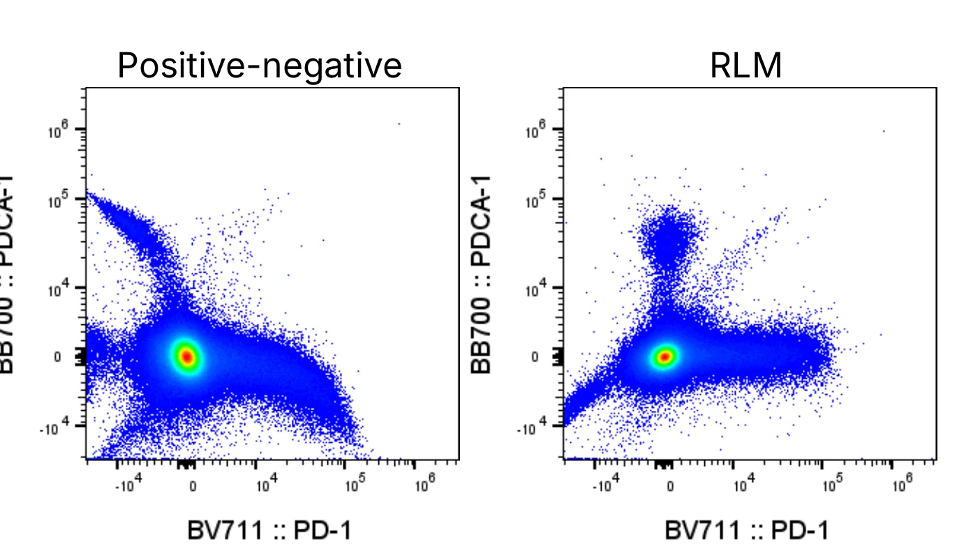
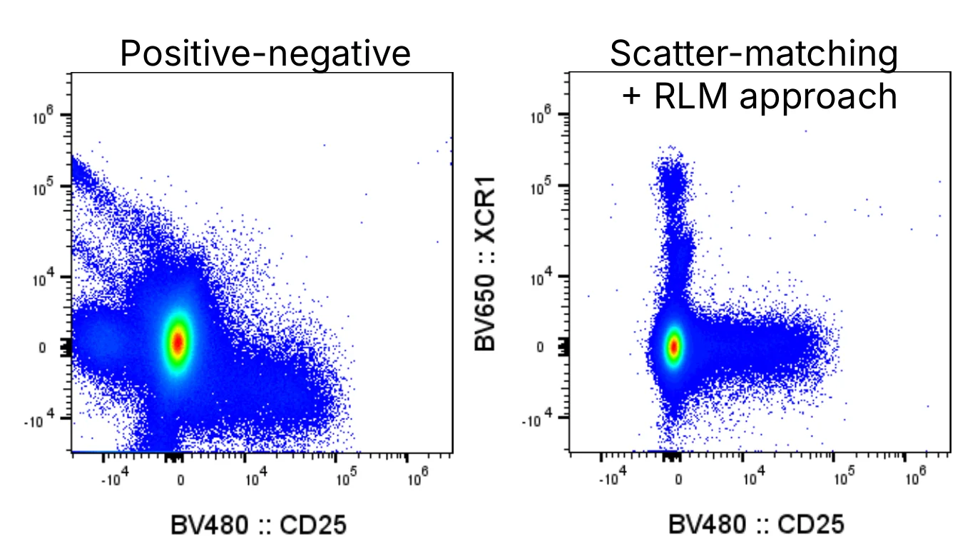
In Honeychrome, these steps run when you click Clean Controls in the Spectral Process.

2. Autofluorescence, cell by cell

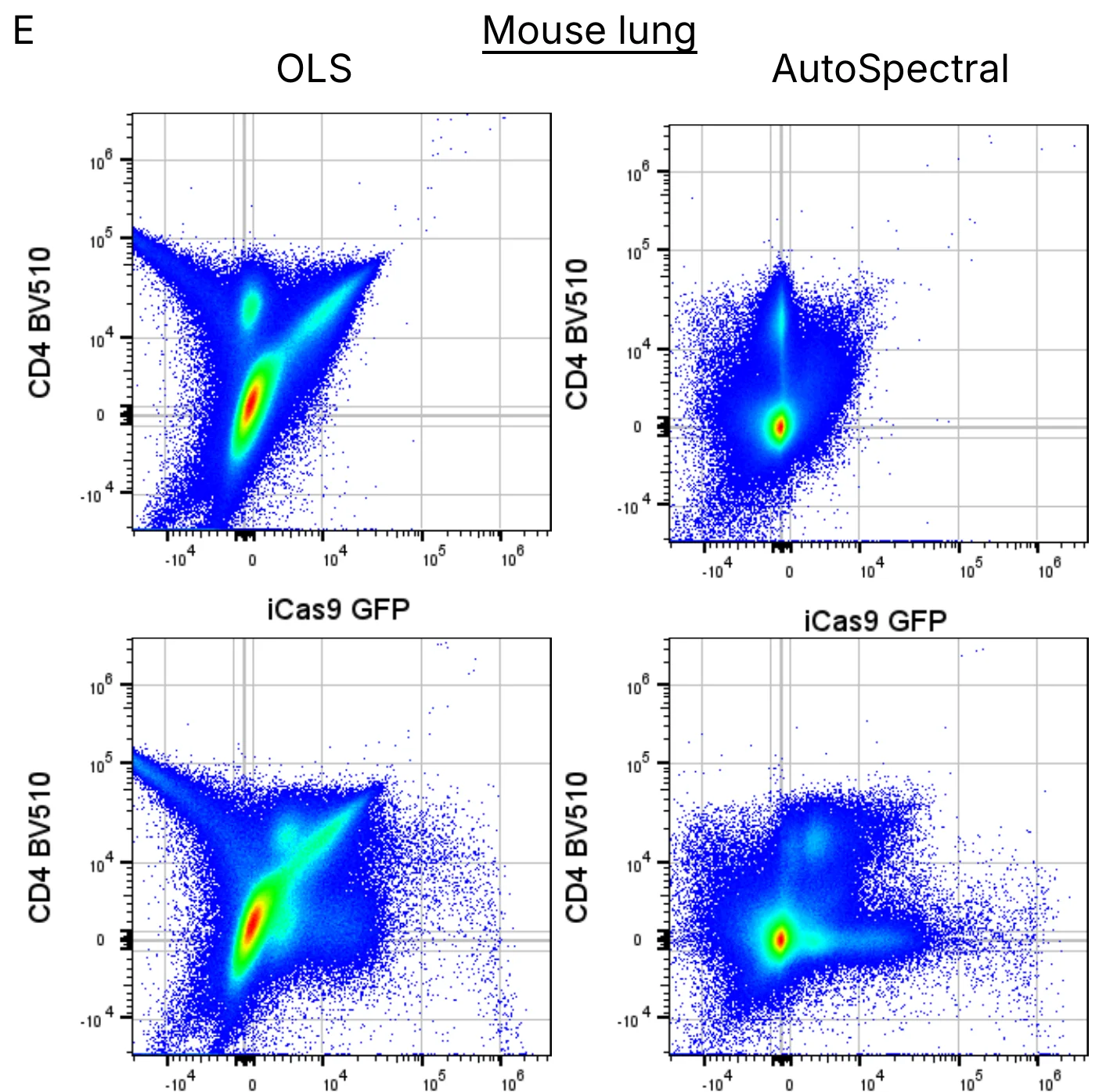
The unstained sample is mapped onto a self-organising map (Kohonen 1995; Van Gassen et al. 2015), and the nodes become a library of candidate autofluorescence spectra. Each cell is then refitted against every candidate. The chosen spectrum is the one that best minimises the product of two ratios: the residual left after subtracting it, and the change it causes in the fluorophore channels. Because every cell is scored on its own, a rare spectrum is scored exactly as a common one, and a cell’s result does not depend on the other cells in the file.

The identity of each cell’s spectrum is written out as the AF Index channel. In the study it tracked scatter, cell type and imaging parameters, so it can be useful biology in its own right (Pilkington 2024).

Mouse lung, 42-colour panel: no AF extraction, one AF spectrum, several AF spectra, and AutoSpectral per-cell AF. Burton et al. 2025, Figure 6E.

3. Fluorophore variation, cell by cell

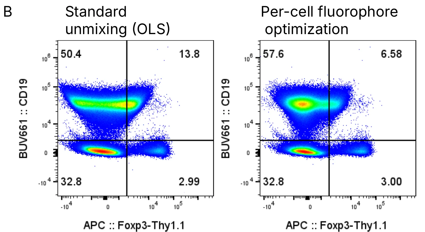
Each single-stained control is mapped in the same way to give a set of spectral variants for its fluorophore. For each cell, and for each fluorophore that cell clearly carries, the variant that most reduces the residual without leaking signal into other channels is chosen. Each change is checked against the cell’s residual and undone if it does not help. This reduces spillover spread between similar dyes and the skews that appear when a control’s spectrum differs from the sample’s.

Per-cell fluorophore optimisation halves the false CD19+ Foxp3+ events caused by BUV661 spread into APC (13.8% to 6.58%). Burton et al. 2025, Figure 7B.

A weak GFP reporter in mouse lung. With ordinary least squares, spread and diagonal spikes hide the signal; with AutoSpectral, the wild-type mouse (top) is clean and GFP+ T cells are resolved in the reporter mouse (bottom). Burton et al. 2025, Figure 7E.

What the study found

AutoSpectral was tested on a 42-colour mouse tissue panel (Cytek Aurora), a 40-colour human PBMC panel (Sony ID7000), the 50-colour OMIP-102 (Konecny et al. 2024; BD FACSDiscover S8) and OMIP-095 (Kare et al. 2023). Per-cell autofluorescence extraction reduced the mis-assignment of the most affected cell positions in unstained samples by up to 9000-fold, and spillover error more broadly by 10- to 100-fold. On single-stained controls, where the truth is known, AutoSpectral gave less spread and fewer off-target errors than experienced human operators and FlowJo’s semi-automated workflow.

Because each step is deterministic, the same data always give the same result, whoever runs them.

Limitations

• AutoSpectral needs good controls. It cannot make up for poorly chosen controls, sample preparation or acquisition; if anything, it rewards extra care.
• An autofluorescence spectrum can only be assigned if cells like it are in the unstained sample. In spike-in tests, a population was found reliably once it made up about 0.3% of the unstained sample.
• Per-cell unmixing is slower than a single least-squares fit, though a fully stained 42-colour lung sample takes about as long to unmix as to acquire.

New methods in Honeychrome 1.0

These methods are new and not yet published. The help on each page of the app describes the settings in full.

• Noise-weighted unmixing and spectral correction were developed for Honeychrome and are not covered in the AutoSpectral manuscript. Both are optional; spectral correction is in beta testing.
• Automated Gating and Flow Set Enrichment Analysis: manuscripts in preparation.

Noise-weighted unmixing

Every detector reads with noise: a constant electronic floor plus photon noise that grows with the signal. The optional noise model, fitted to your controls, weights each detector by how noisy it is. A positivity prior pulls fluorophores that a cell is clearly negative for towards zero, so their spread no longer lands in other channels. This builds on Poisson-based unmixing (Novo et al. 2013) and on removing irrelevant dyes from each cell’s fit (Kmet and Novo 2025), and was shaped by work with Paul Heisig (Amsterdam UMC) and David Novo.

Spectral correction (beta testing)

A reference spectrum can still be slightly wrong for fully stained cells: a tandem that has degraded differently, a control stained on beads, a different buffer. In a fully stained sample, cells negative for a marker should read zero, so leftover spillover shows as negative cells drifting with another marker. Spectral correction measures that drift and corrects the spectra, including through a tandem’s parent dye when the tandem has broken down. Tools such as CompensAID (Olsman et al. 2026) detect these reference errors; spectral correction also fixes them.

Automated Gating (manuscript in preparation)

Automated Gating turns a gating strategy, from Honeychrome or a FlowJo workspace, into data-driven gates that are trained once and then applied to every sample. Thresholds come from the tail of the negative population or from mixture models, and a cells gate from the fall-off of scatter density. Each gate can stay fixed or be recalculated for each sample. Automated gating methods have been published before (Finak et al. 2014; Malek et al. 2015); this one was developed in the Liston-Dooley lab, and its R implementation is the AutoGating package.

Flow Set Enrichment Analysis (manuscript in preparation)

Flow Set Enrichment Analysis asks whether the populations of a known cell type move together between groups of samples, in the manner of gene set enrichment analysis (Subramanian et al. 2005), using curated human and mouse cell-type libraries. It is on the Enrichment page of Automated Gating.

Workflows built on published methods

Honeycluster and the statistics shared by Honeycluster and Automated Gating were developed for Honeychrome from existing, published methods. They run on the same unmixed data, gates and sample groups as the rest of the app; the references below are the ones each part follows.

Honeycluster

Honeycluster combines dimensionality reduction (UMAP, t-SNE, PaCMAP, PCA), clustering (FlowSOM, HDBSCAN, Leiden) and automatic annotation. Cluster labels come from marker enrichment modelling (Diggins et al. 2017) and ScType-style scoring (Ianevski et al. 2022) against a curated cell-type and marker database.

Statistics

Honeycluster and Automated Gating share one statistics engine:

• Differential abundance uses count models with a quasi-likelihood F test (Lund et al. 2012) and an adjustment for small counts (Chen et al. 2025), as in edgeR.
• Differential expression uses moderated linear models (Smyth 2004; Ritchie et al. 2015), with optional fold-change thresholds (McCarthy and Smyth 2009).
• Clusters and populations are tested one by one, as in diffcyt (Weber et al. 2019), and the false discovery rate is controlled across families of tests (Benjamini and Bogomolov 2014).

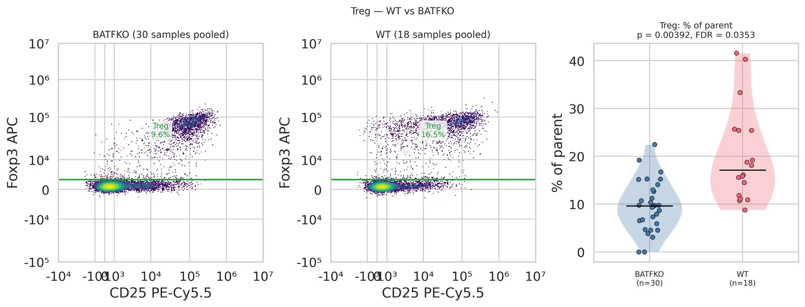
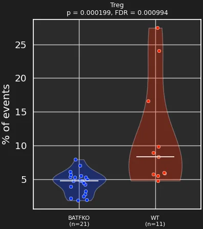
So the same question can be asked of gated populations and of clusters. In the BATF chimera dataset (PMID 38897202), Tregs are less frequent in the BATFKO group than in the WT group, whether they are defined by Automated Gating or found as a Honeycluster cluster.

Treg frequency, BATFKO against WT. Automated Gating: each group’s pooled events with the Treg gate, and Tregs as a percentage of their parent population in 48 samples (p = 0.0039, FDR = 0.035). Honeycluster: the Treg cluster as a percentage of clustered events in 32 samples (p = 0.0002, FDR = 0.001). Data from PMID 38897202.

How to cite

If you used the AutoSpectral workflows (control cleaning, per-cell autofluorescence, spectral variants), please cite:

Burton OT, Laniewski N, Rogers SS, Lopez Munoz-de-Leon A, Khan S, Arunthavalingam J, Smith E, Bücken L, De Vuyst L, Humblet-Baron S, Cerveira J, Scheible K, Dooley J, Liston A. AutoSpectral improves spectral flow cytometry accuracy through optimised spectral unmixing and autofluorescence-matching at the cellular level. bioRxiv 2025. doi:10.1101/2025.10.27.684855

Noise-weighted unmixing, spectral correction, Automated Gating and Flow Set Enrichment Analysis are not yet published. If you used them, name them and the Honeychrome version in your methods.

Please also name Honeychrome and its version in your methods, with a link to honeychrome.cytkit.com, and cite the methods you used from the references below.

Data and code

• Example data for the Spectral unmixing guide: the AutoSpectral Full Workflow Example.
• Data from the AutoSpectral study on Mendeley Data: 42-colour mouse tissue doi:10.17632/y2zp5xx2hg.2 (AutoSpectral unmixed: doi:10.17632/vzdxy8n7wf.1); 7-colour mouse liver doi:10.17632/ch5dnspd79.1; mouse brain imaging doi:10.17632/9nsk2tcjsz.1; 40-colour human PBMC, ID7000 doi:10.17632/2kvc98hc65.1; autofluorescence spike-in doi:10.17632/njb5zkyjp6.1.
• AutoSpectral R package: github.com/DrCytometer/AutoSpectral, and the faster per-cell version AutoSpectralRcpp.
• Articles on AutoSpectral, unmixing and analysis on the Colibri Cytometry blog.
• Honeychrome source code: github.com/Cytkit/honeychrome.

References

Unmixing and autofluorescence

1. Burton OT et al. AutoSpectral improves spectral flow cytometry accuracy through optimised spectral unmixing and autofluorescence-matching at the cellular level. bioRxiv 2025. doi:10.1101/2025.10.27.684855
2. Roca CP et al. AutoSpill is a principled framework that simplifies the analysis of multichromatic flow cytometry data. Nat Commun 2021;12:2890. doi:10.1038/s41467-021-23126-8
3. Roederer M. Compensation in flow cytometry. Curr Protoc Cytom 2002;Unit 1.14. doi:10.1002/0471142956.cy0114s22
4. Roederer M. Distributions of autofluorescence after compensation: be Panglossian, fret not. Cytometry A 2016;89(4):398–402. doi:10.1002/cyto.a.22820
5. Novo D, Grégori G, Rajwa B. Generalized unmixing model for multispectral flow cytometry utilizing nonsquare compensation matrices. Cytometry A 2013;83(5):508–520. doi:10.1002/cyto.a.22272
6. Novo D. A comparison of spectral unmixing to conventional compensation for the calculation of fluorochrome abundances from flow cytometric data. Cytometry A 2022;101(11):885–891. doi:10.1002/cyto.a.24669
7. Kmet R, Novo D. Reducing spreading: removing the impact of irrelevant dyes improves unmixed flow cytometry data. Cytometry A 2025. doi:10.1002/cyto.a.24957
8. Nguyen R, Perfetto S, Mahnke YD, Chattopadhyay P, Roederer M. Quantifying spillover spreading for comparing instrument performance and aiding in multicolor panel design. Cytometry A 2013;83(3):306–315. doi:10.1002/cyto.a.22251
9. Mage PL, Konecny AJ, Mair F. Measurement and prediction of unmixing-dependent spreading due to collinearity in spectral flow cytometry. Cytometry A 2026;109(6):436–455. doi:10.1002/cyto.a.70044
10. Cai X, Garcia-Garcia S, Kuhnen L, Gianniou M, Garcia Vallejo JJ. Unmixing spread estimation based on residual model in spectral flow cytometry. bioRxiv 2026. doi:10.64898/2026.01.27.701929
11. Ferrer-Font L et al. Panel optimization for high-dimensional immunophenotyping assays using full-spectrum flow cytometry. Curr Protoc 2021;1(9):e222. doi:10.1002/cpz1.222
12. Pilkington KR. Autofluorescence: from burden to benefit. Cytometry A 2024;105(8):563–567. doi:10.1002/cyto.a.24885
13. Olsman R et al. CompensAID: an automated detection tool for reference errors. Cytometry A 2026;109(2):124–134. doi:10.1002/cyto.a.70016
14. Kohonen T. Self-organizing maps. Springer, 1995.

Datasets

1. Konecny AJ, Mage PL, Tyznik AJ, Prlic M, Mair F. OMIP-102: 50-color phenotyping of the human immune system with in-depth assessment of T cells and dendritic cells. Cytometry A 2024;105(6):430–436. doi:10.1002/cyto.a.24841. Data kindly provided by Florian Mair.
2. Kare AJ, Nichols L, Zermeno R, Raie MN, Tumbale SK, Ferrara KW. OMIP-095: 40-color spectral flow cytometry delineates all major leukocyte populations in murine lymphoid tissues. Cytometry A 2023;103(11):839–850. doi:10.1002/cyto.a.24788. Data kindly provided by Debajit Bhowmick.

Gating and transforms

1. Parks DR, Roederer M, Moore WA. A new “Logicle” display method avoids deceptive effects of logarithmic scaling for low signals and compensated data. Cytometry A 2006;69(6):541–551. doi:10.1002/cyto.a.20258
2. Otsu N. A threshold selection method from gray-level histograms. IEEE Trans Syst Man Cybern 1979;9(1):62–66. doi:10.1109/TSMC.1979.4310076
3. Finak G et al. OpenCyto: an open source infrastructure for scalable, robust, reproducible, and automated, end-to-end flow cytometry data analysis. PLoS Comput Biol 2014;10(8):e1003806. doi:10.1371/journal.pcbi.1003806
4. Malek M et al. flowDensity: reproducing manual gating of flow cytometry data by automated density-based cell population identification. Bioinformatics 2015;31(4):606–607. doi:10.1093/bioinformatics/btu677
5. Saeys Y, Van Gassen S, Lambrecht BN. Computational flow cytometry: helping to make sense of high-dimensional immunology data. Nat Rev Immunol 2016;16:449–462. doi:10.1038/nri.2016.56
6. Cheung M et al. Current trends in flow cytometry automated data analysis software. Cytometry A 2021;99(10):1007–1021. doi:10.1002/cyto.a.24320
7. Liu et al. 2025, Briefings in Bioinformatics (evaluation of gating methods). doi:10.1093/bib/bbae633

Dimensionality reduction, clustering and annotation

1. McInnes L, Healy J, Melville J. UMAP: Uniform Manifold Approximation and Projection for dimension reduction. arXiv 2018. arXiv:1802.03426
2. van der Maaten L, Hinton G. Visualizing data using t-SNE. J Mach Learn Res 2008;9:2579–2605. jmlr.org
3. Poličar PG, Stražar M, Zupan B. openTSNE: a modular Python library for t-SNE dimensionality reduction and embedding. J Stat Softw 2024;109(3). doi:10.18637/jss.v109.i03
4. Wang Y, Huang H, Rudin C, Shaposhnik Y. Understanding how dimension reduction tools work: an empirical approach to deciphering t-SNE, UMAP, TriMap, and PaCMAP for data visualization. J Mach Learn Res 2021;22(201):1–73. arXiv:2012.04456
5. Van Gassen S et al. FlowSOM: using self-organizing maps for visualization and interpretation of cytometry data. Cytometry A 2015;87(7):636–645. doi:10.1002/cyto.a.22625
6. Traag VA, Waltman L, van Eck NJ. From Louvain to Leiden: guaranteeing well-connected communities. Sci Rep 2019;9:5233. doi:10.1038/s41598-019-41695-z
7. Campello RJGB, Moulavi D, Sander J. Density-based clustering based on hierarchical density estimates. PAKDD 2013. doi:10.1007/978-3-642-37456-2_14
8. Diggins KE, Greenplate AR, Leelatian N, Wogsland CE, Irish JM. Characterizing cell subsets using marker enrichment modeling. Nat Methods 2017;14:275–278. doi:10.1038/nmeth.4149
9. Ianevski A, Giri AK, Aittokallio T. Fully-automated and ultra-fast cell-type identification using specific marker combinations from single-cell transcriptomic data. Nat Commun 2022;13:1246. doi:10.1038/s41467-022-28803-w

Statistics

1. Smyth GK. Linear models and empirical Bayes methods for assessing differential expression in microarray experiments. Stat Appl Genet Mol Biol 2004;3:Article 3. doi:10.2202/1544-6115.1027
2. Ritchie ME et al. limma powers differential expression analyses for RNA-sequencing and microarray studies. Nucleic Acids Res 2015;43(7):e47. doi:10.1093/nar/gkv007
3. Robinson MD, McCarthy DJ, Smyth GK. edgeR: a Bioconductor package for differential expression analysis of digital gene expression data. Bioinformatics 2010;26(1):139–140. doi:10.1093/bioinformatics/btp616
4. Lund SP, Nettleton D, McCarthy DJ, Smyth GK. Detecting differential expression in RNA-sequence data using quasi-likelihood with shrunken dispersion estimates. Stat Appl Genet Mol Biol 2012;11(5). doi:10.1515/1544-6115.1826
5. Chen Y, Chen L, Lun ATL, Baldoni PL, Smyth GK. edgeR v4: powerful differential analysis of sequencing data with expanded functionality and improved support for small counts and larger datasets. Nucleic Acids Res 2025;53(2):gkaf018. doi:10.1093/nar/gkaf018
6. McCarthy DJ, Smyth GK. Testing significance relative to a fold-change threshold is a TREAT. Bioinformatics 2009;25(6):765–771. doi:10.1093/bioinformatics/btp053
7. Benjamini Y, Bogomolov M. Selective inference on multiple families of hypotheses. J R Stat Soc B 2014;76(1):297–318. doi:10.1111/rssb.12028
8. Weber LM, Nowicka M, Soneson C, Robinson MD. diffcyt: differential discovery in high-dimensional cytometry via high-resolution clustering. Commun Biol 2019;2:183. doi:10.1038/s42003-019-0415-5
9. Subramanian A et al. Gene set enrichment analysis: a knowledge-based approach for interpreting genome-wide expression profiles. PNAS 2005;102(43):15545–15550. doi:10.1073/pnas.0506580102

Software

1. White S et al. FlowKit: a Python toolkit for integrated manual and automated cytometry analysis workflows. Front Immunol 2021;12:768541. doi:10.3389/fimmu.2021.768541