Spectral unmixing

Create an experiment, import FCS files, build a spectral model from single-stained controls, then unmix and check the result.

This guide takes you from FCS files to unmixed data. It uses the AutoSpectral Full Workflow Example, a 9-colour panel run on a 5-laser Cytek Aurora. To follow along, download the data from the AutoSpectral Full Workflow Example post (it links to the files on Mendeley Data) and unzip them. If you have not installed Honeychrome yet, see Install.

Create an experiment

Start Honeychrome and choose New Experiment. Type a name, for example “AutoSpectral Full Workflow Example”. This creates a .kit file, which holds the experiment’s settings, and a folder of the same name for the FCS files, exports and reports.

Honeychrome start-up screen with New Experiment and Open Experiment

Import your FCS files

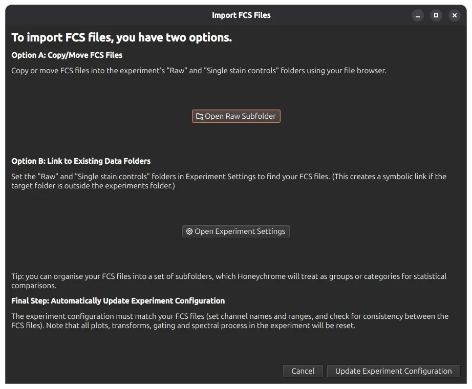
Choose File > Import FCS Files. You can either copy or move your FCS files into the experiment’s Raw folder, or link to an existing data folder.

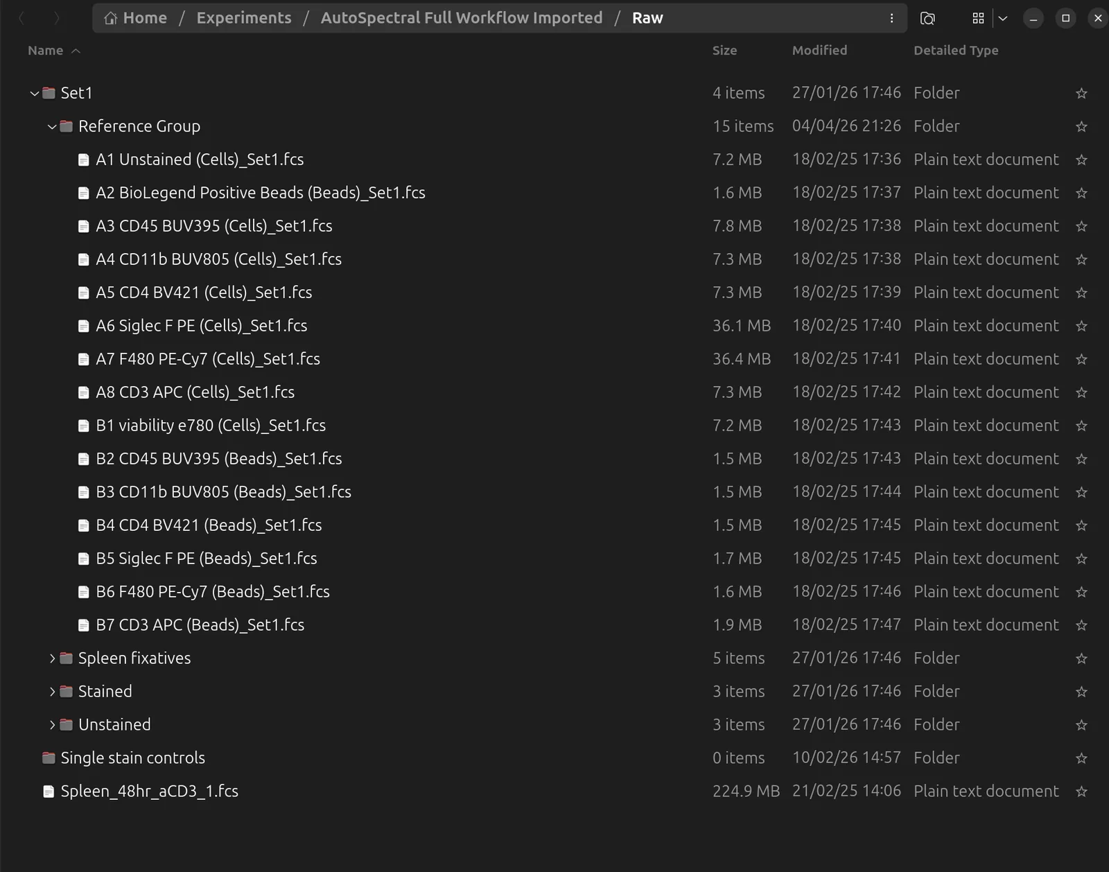
Import FCS Files dialog offering to copy, move or link FCS files into the Raw folder

Honeychrome keeps the folder structure of your files and shows the same folders in the sample browser on the left. Folders are also used as sample groups later, for example in Simple Stats and when assigning autofluorescence profiles.

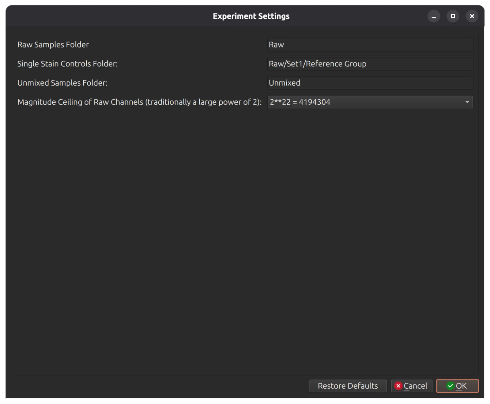
Sample browser showing the imported FCS files grouped by their folders

Tell Honeychrome where the single-stained controls are. Open Edit > Experiment Settings (or use the button in the import dialog) and click single stained controls to choose the folder.

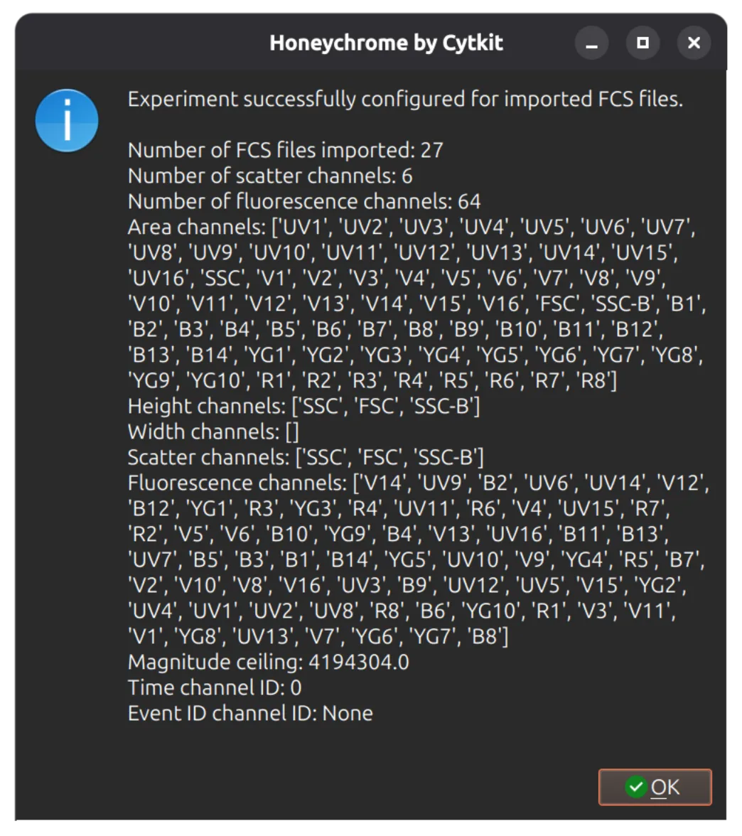
Experiment Settings with the single stained controls folder selected

Then click Update Experiment Configuration at the bottom of the dialog. Honeychrome reads the channels of every file and checks that they are consistent. If the detector voltages or gains differ between files, it warns you, because Honeychrome does not adjust for them.

Update Experiment Configuration button at the bottom of the Experiment Settings dialog

Check the raw data

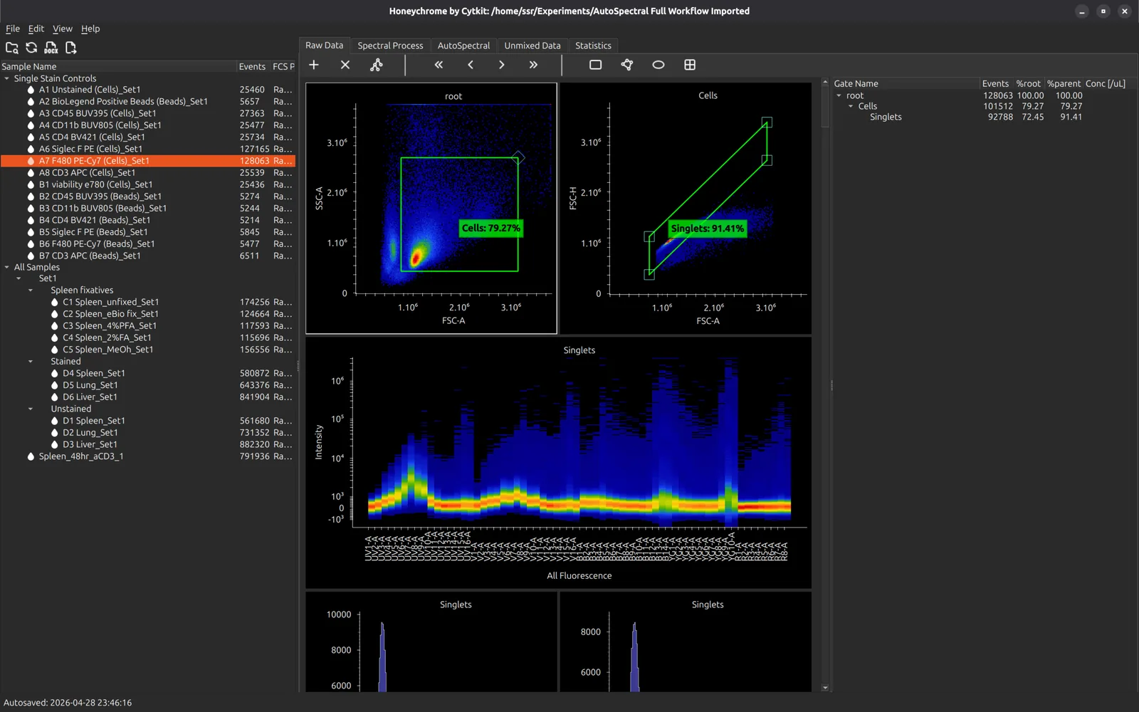
Click any sample in the sample browser to load it. The Raw Data tab shows morphology plots, a ribbon plot of every detector, and histograms.

Set broad scatter gates here that keep every cell of interest, large and small, but not doublets. The spectral controls use them.

You can draw gates on the raw data, but do your analysis in the Unmixed Data tab, once the spectral model is built.

Raw Data tab with morphology plots, a ribbon plot and histograms for the selected sample

Unstained and bead samples

The sample browser marks two kinds of sample, and you can change either with a right click:

Unstained samples have a blue droplet icon. Files with “unstained” in the name are recognised automatically. Use Mark as Unstained or Unmark as Unstained for others.
Bead samples are shown in green. Unstained samples and single-stained controls whose scatter looks like beads are marked automatically. Use Mark as Beads or Unmark as Beads to correct it; your choice is final.

Unstained, single-stained and bead samples are left out by default when you choose samples for analysis.

Build the spectral model

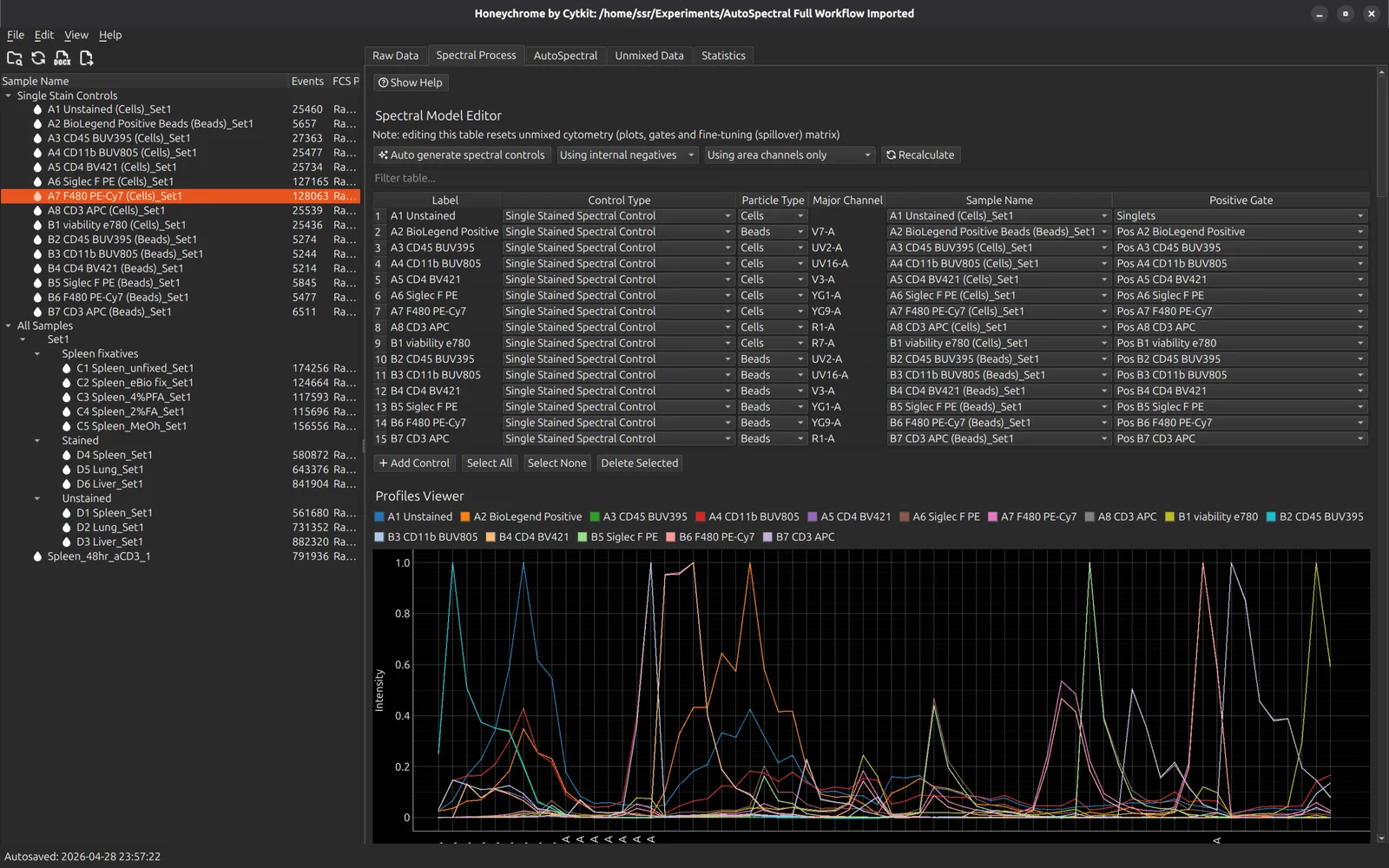
Open the Spectral Process tab and press Auto generate spectral controls. Honeychrome makes one control for each file in the single-stained controls folder:

The label comes from the start of the file name, and antigen and fluorophore names are recognised.
The particle type comes from the name, for example “CD4 BUV395 (Cells)” or “(Beads)”. When the name does not say, Honeychrome decides from the scatter, and bead controls are matched to the right unstained bead sample when there are several bead types.
The major channel is the detector where the fluorophore varies most. A positive gate is placed on the brightest events and a negative gate on the dimmest (5% and 25% by default, set in App Configuration). The gates are added to the raw data plots, where you can adjust them.

Spectral Process tab after Auto generate spectral controls, listing a control for each FCS file

Choose the negative

Each spectrum is the mean of the positive events minus a negative:

Using internal negatives (the default) takes the dimmest events of the same control.
Using unstained negative takes an unstained sample instead, which is usually better. Choose the unstained sample for each control in the Unstained Negative column, or for all at once with Set negative for all.

With an unstained negative and Automatically Clean ticked (the default), AutoSpectral control cleaning runs straight after the controls are generated. See Control cleaning.

Tidy the controls

This example has both cell and bead controls for some fluorophores. Select the bead controls and press Delete Selected. You can also rename labels here, or go back to the Raw Data tab and adjust the gates of a control.

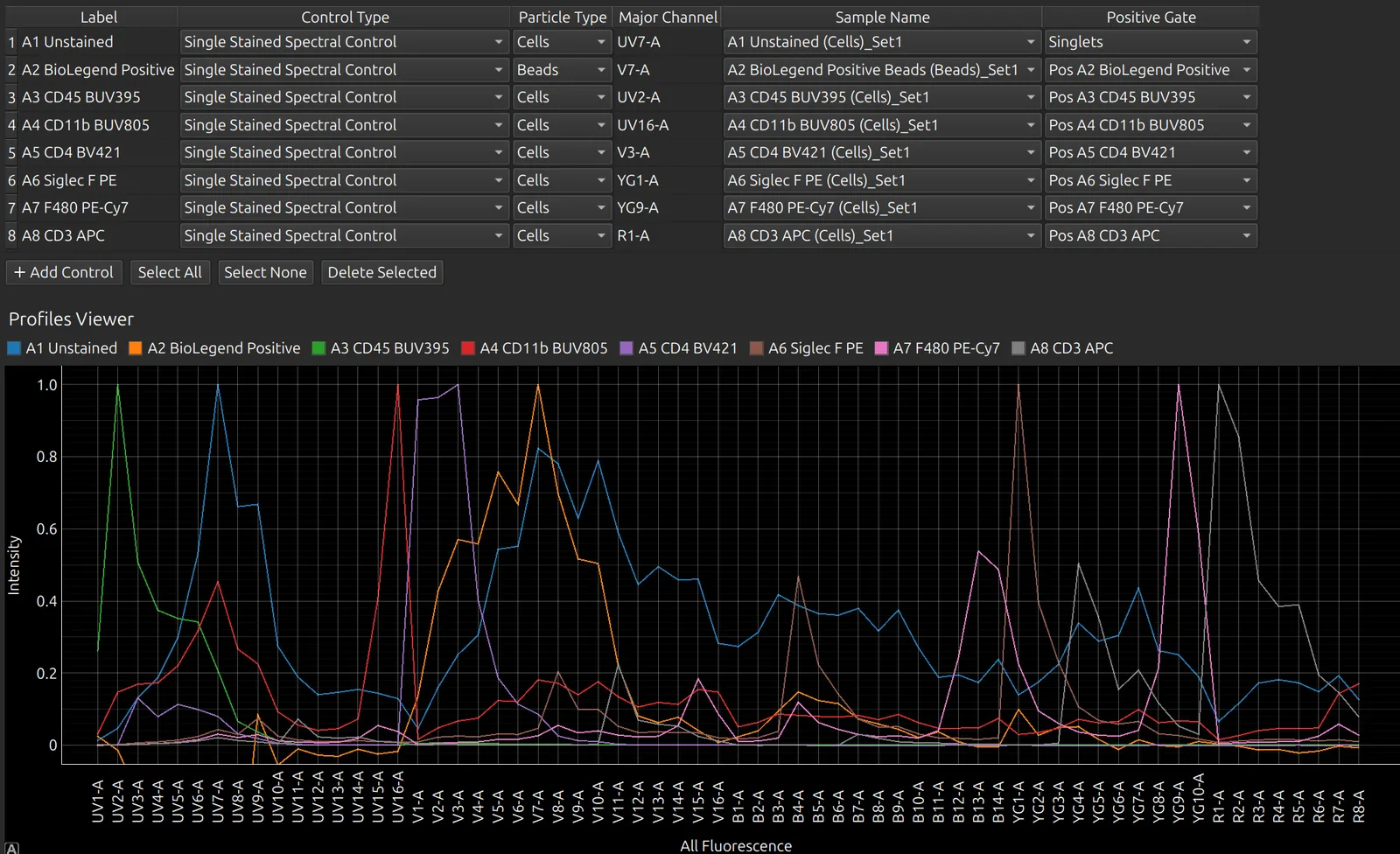
Spectral model editor after deleting the duplicate bead controls

If you change the sample of a control, for example from cells to beads, its particle type and negative follow the new sample. Its gates are placed again, and it is cleaned again if Automatically Clean is on.

Unmixed gates are kept when the spectral model is regenerated.

Use a spectrum from the Reference Library

If a control has failed, use a spectrum from the Reference Library instead:

Set the control’s Control Type to Single Stained Spectral Control from Library.
Enter the fluorophore as the label.
Choose a match under Sample Name. Only spectra recorded on the same instrument and detector configuration are offered.

To add one of your own controls to the library, right-click it in the spectral model editor and choose Save to Reference Library. View > Reference Library opens the library itself, where you can browse, compare, import and export spectra for your instrument.

Check the spectral model

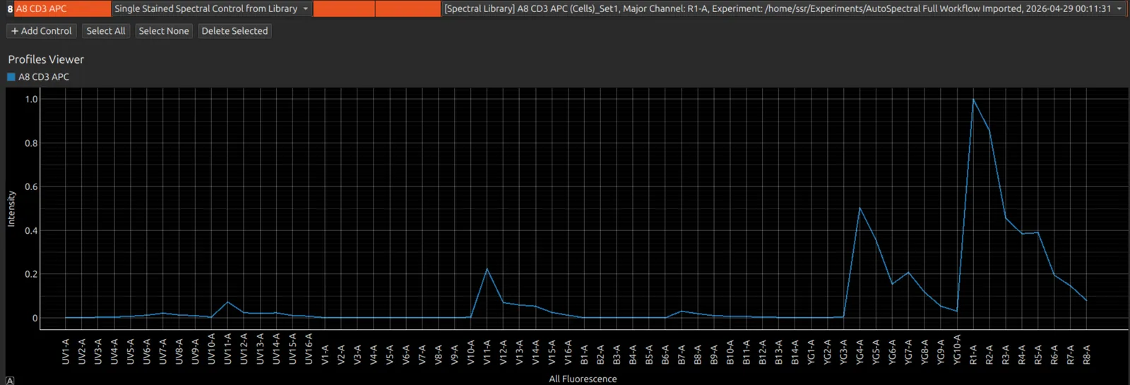
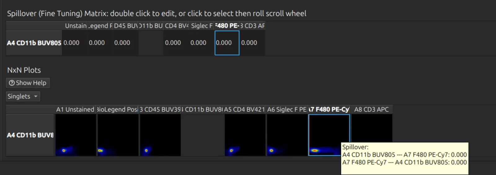
Select one or more controls in the table to show only their spectra, and only their rows of the matrices and NxN plots. This makes large panels much easier to work with.

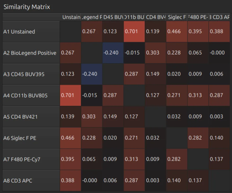
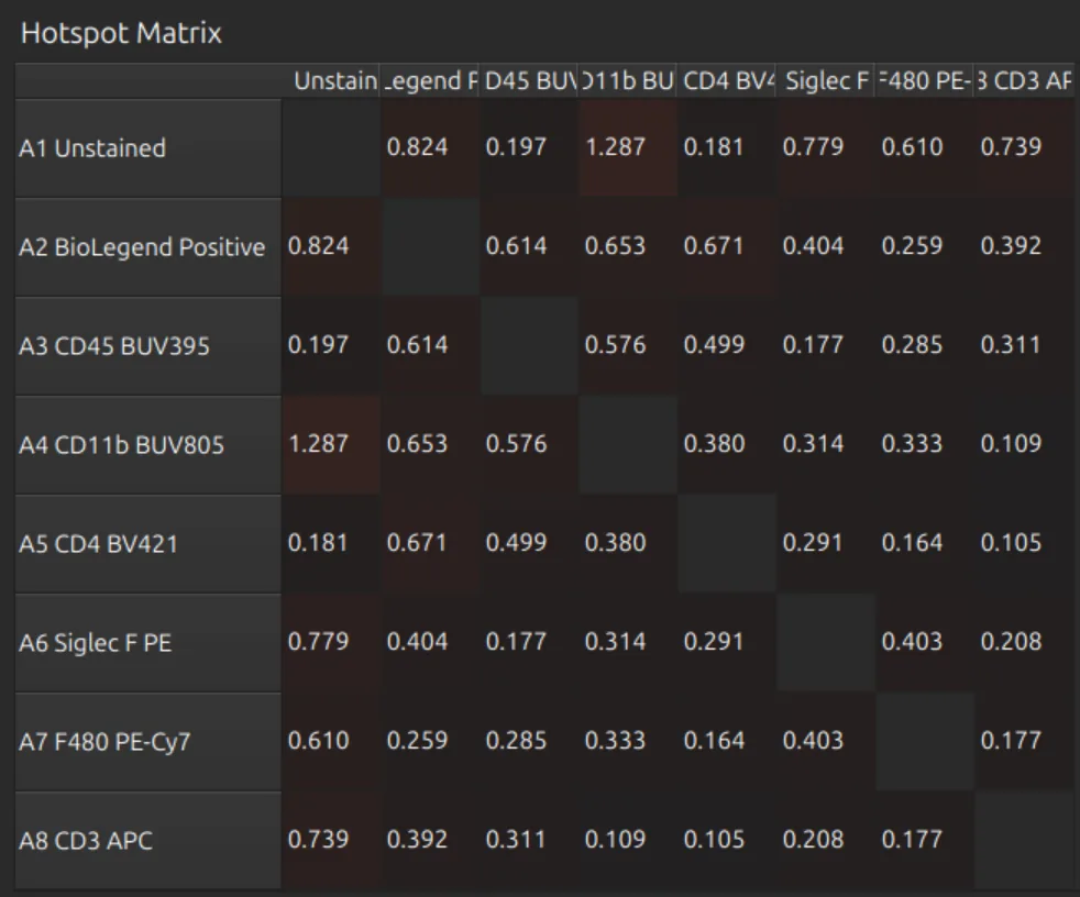
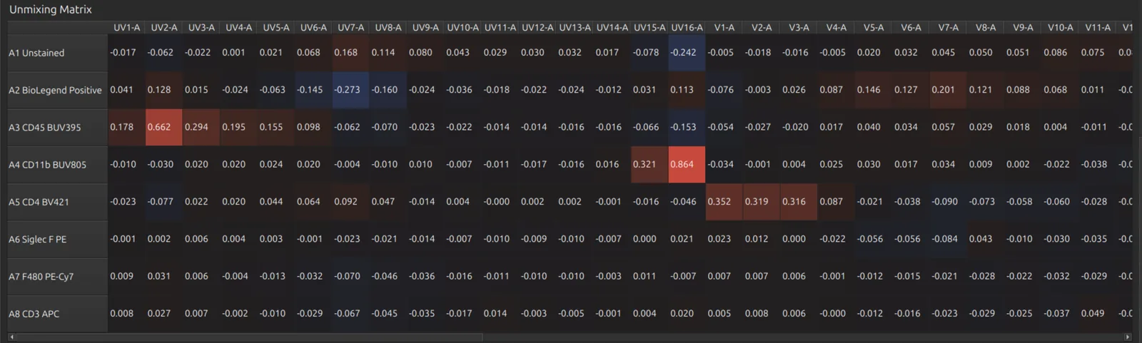
Press Select None (or Select All) to see every spectrum and the full matrices:

the similarity matrix: how alike each pair of spectra is;
the hotspot matrix: where unmixing will spread signal between fluorophores;
the unmixing matrix.

The condition number of the spectral model is shown above the table. Higher values mean less stable unmixing, and Honeychrome warns about a poorly conditioned matrix.

Similarity matrix of the fluorophore spectra

Hotspot matrix of the fluorophore spectra

Fine tune

The spillover matrix and the NxN plots let you fine tune the unmixing by hand. The NxN plots show every pair of unmixed labels for the sample selected in the sample browser.

Click a cell of the spillover matrix or a tile of the NxN plots, then roll the mouse wheel to adjust it. You must click first, so scrolling the page cannot change the spillover by accident.
Double-click a cell of the spillover matrix to type a value.
Hover over a tile to see its spillover.

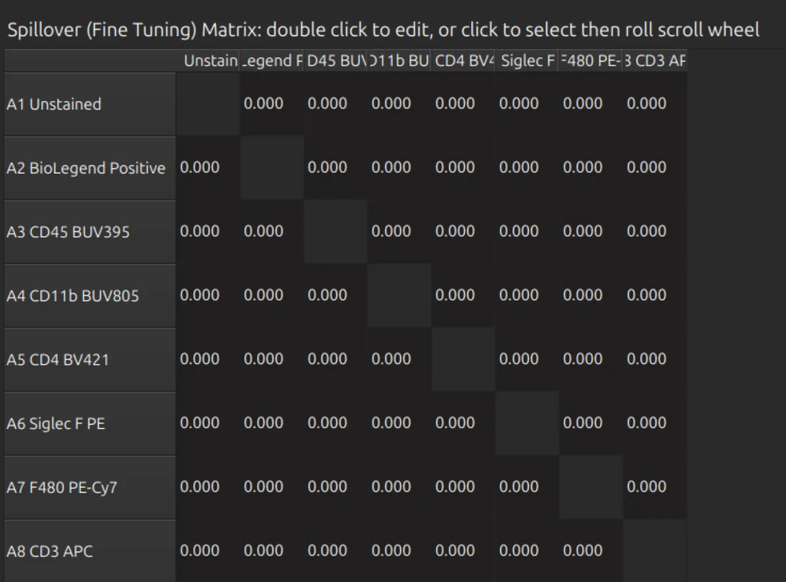
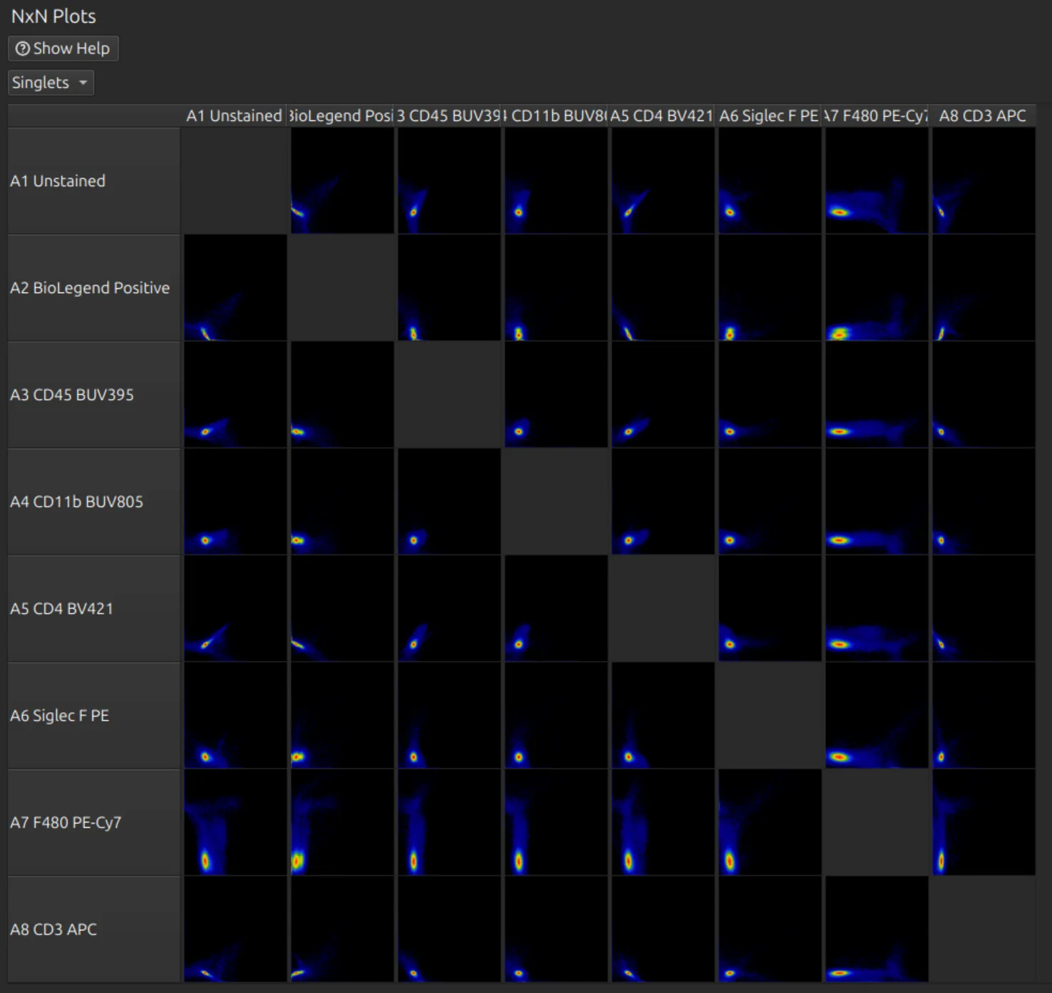
NxN plots of every pair of unmixed labels

With a large panel, select the labels you are working on first. With nothing selected, every pair is drawn: a 60-colour panel means 1,800 plots at once.

Fine tuning with only the selected labels shown in the spillover matrix and NxN plots

Analyse the unmixed data

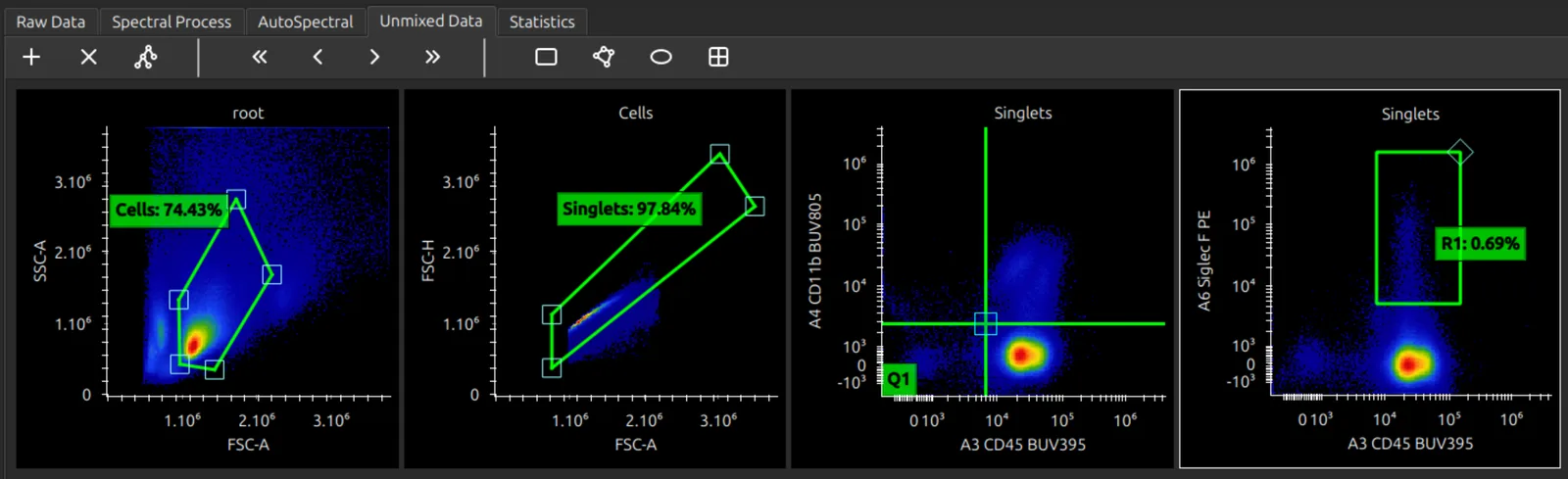
Open the Unmixed Data tab to analyse your unmixed data; see Plots and gates.

Unmixed Data tab with plots of the unmixed labels

Next steps

AutoSpectral in Honeychrome: clean the controls and remove autofluorescence cell by cell.
Plots and gates
Simple Stats and Reports and exports

Spectral unmixing

Create an experiment

Import your FCS files

Check the raw data

Unstained and bead samples

Build the spectral model

Choose the negative

Tidy the controls

Use a spectrum from the Reference Library

Check the spectral model

Fine tune

Analyse the unmixed data

Next steps

Further reading