Autofluorescence

Give every cell its own best-fitting autofluorescence spectrum, so autofluorescence stops appearing as false signal in your markers.

Autofluorescence differs between cell types, tissues and preparations, so a single autofluorescence spectrum, or none, is wrong for most cells in a mixed sample. The Autofluorescence page of the AutoSpectral tab builds a library of autofluorescence spectra from each unstained sample. Each cell is then unmixed with the spectrum from that library that fits it best.

You need at least one unstained sample, marked as unstained (see Control cleaning). Ideally have one for each tissue or preparation in the experiment.

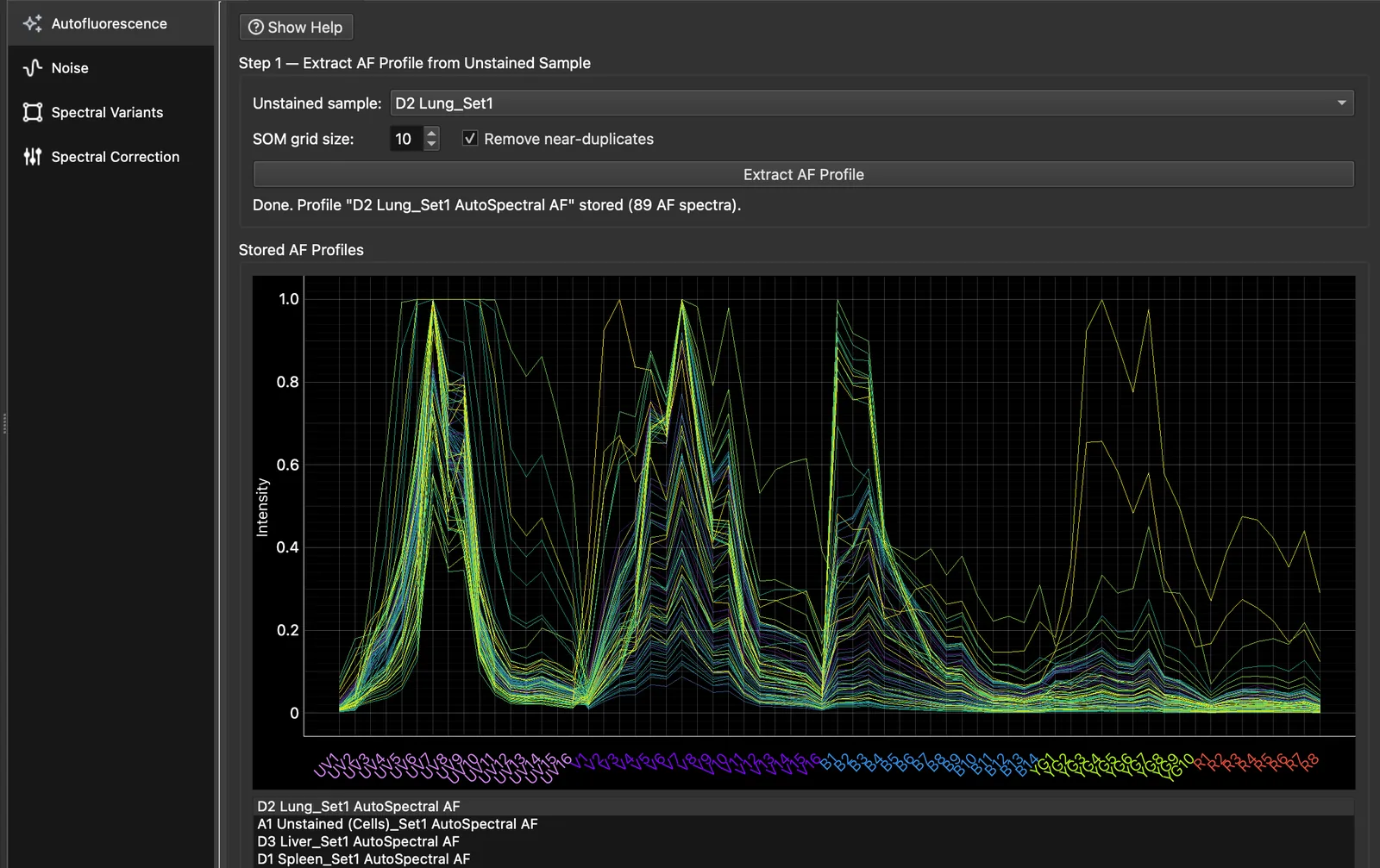
Step 1: extract an AF profile from each unstained sample

Under Step 1, choose an unstained sample. Only samples marked as unstained are listed.
Press Extract AF Profile. The sample’s autofluorescence is clustered on a self-organising map: a SOM grid size of 10 gives at most 100 spectra. Near-duplicates are removed, so you usually see fewer.
Repeat for each unstained sample, for example one per tissue. Each gives one AF profile.

Click a profile under Stored AF Profiles to see its spectra; the profile mean is drawn in black.

To remove one spectrum (for example one that is clearly a fluorophore, not autofluorescence), right-click it in the plot and choose Delete spectrum…. The mean cannot be deleted.
Delete Selected removes a whole profile and its assignments.
Profiles can be saved to and loaded from CSV.

Deleting a spectrum renumbers the experiment’s AF Index, so a gate drawn on AF Index may select different spectra afterwards. Extract the profile again to restore it.

Step 1 on the unstained lung sample of the AutoSpectral Full Workflow Example: 89 autofluorescence spectra from a 10 × 10 map. One profile is stored for each unstained sample.

Step 2: assign profiles to samples

Each row of the Step 2 grid is a sample and each column an AF profile. Tick the profiles for each sample; a sample can have more than one. Each cell of the sample then gets the best-fitting spectrum from all of its ticked profiles.

To assign many samples at once:

select a profile under Stored AF Profiles and press Assign Selected Profile to All Samples;
or choose a folder and press Assign Selected Profile to Folder, which assigns every sample shown in that folder and its subfolders.

Unstained and single-stained controls are hidden from the grid; tick Include unstained controls or Include single-stained controls to show them.

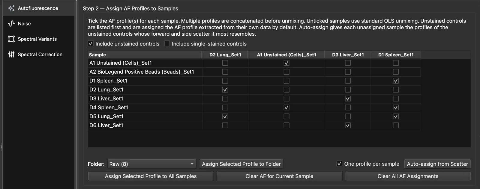
Autofluorescence page, Step 2: a grid of samples against AF profiles, with the assignment buttons below — Step 2: samples (rows) against AF profiles (columns). A sample can take more than one profile.

Auto-assign from scatter

Auto-assign from Scatter fills in the samples in the grid that have no profile yet. It skips bead samples and never changes an existing assignment.

The forward and side scatter of each unstained sample with a profile is modelled as a Gaussian mixture.
Each sample is given the profile of the unstained sample whose scatter best explains its own.
With One profile per sample ticked (the default), each sample gets one profile. Unticked, up to three are chosen by BIC. A second or third is added only when it improves the fit and accounts for at least 30% of the events.

A summary opens at the end. Show Details lists first the samples whose scatter lies partly outside every unstained sample assigned to them.

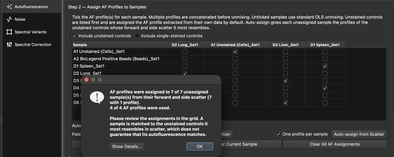
Auto-assign summary: AF profiles were assigned to 7 of 7 unassigned samples from their forward and side scatter, and 4 of 4 profiles were used — The summary after Auto-assign from Scatter.

Review the assignments before you analyse. Similar scatter does not guarantee similar autofluorescence.

Step 3: compare

Step 3 shows the current sample unmixed by ordinary least squares without autofluorescence (left) and with per-cell AF (right). Assigned to sample uses the Step 2 assignment; choosing a single profile previews it without changing the assignment.

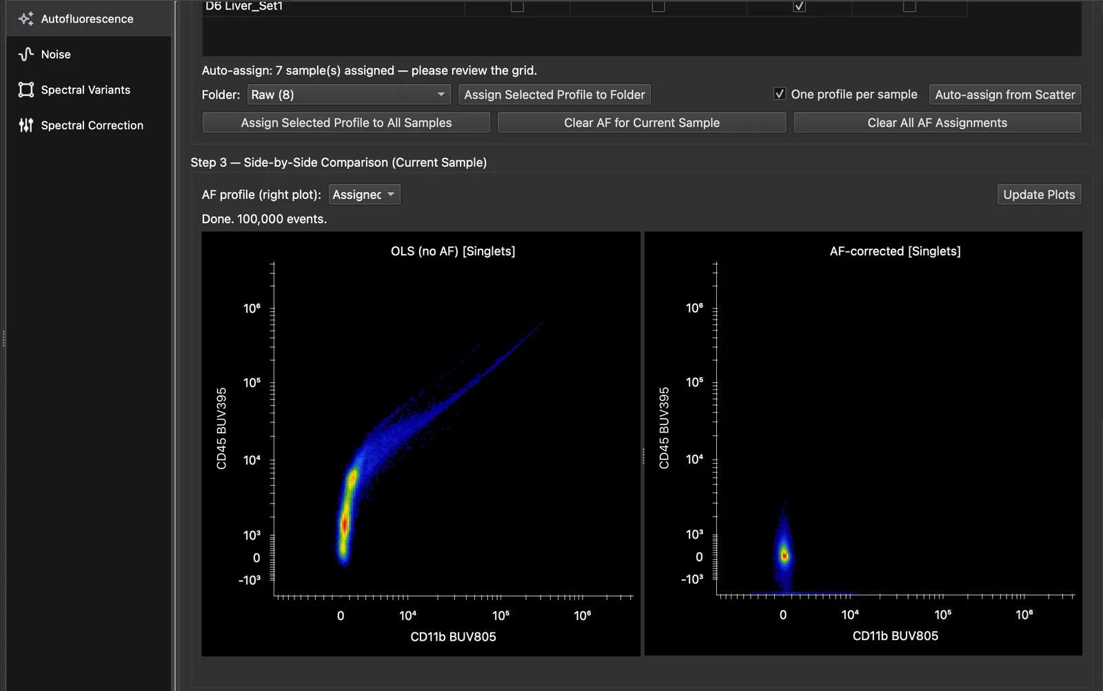
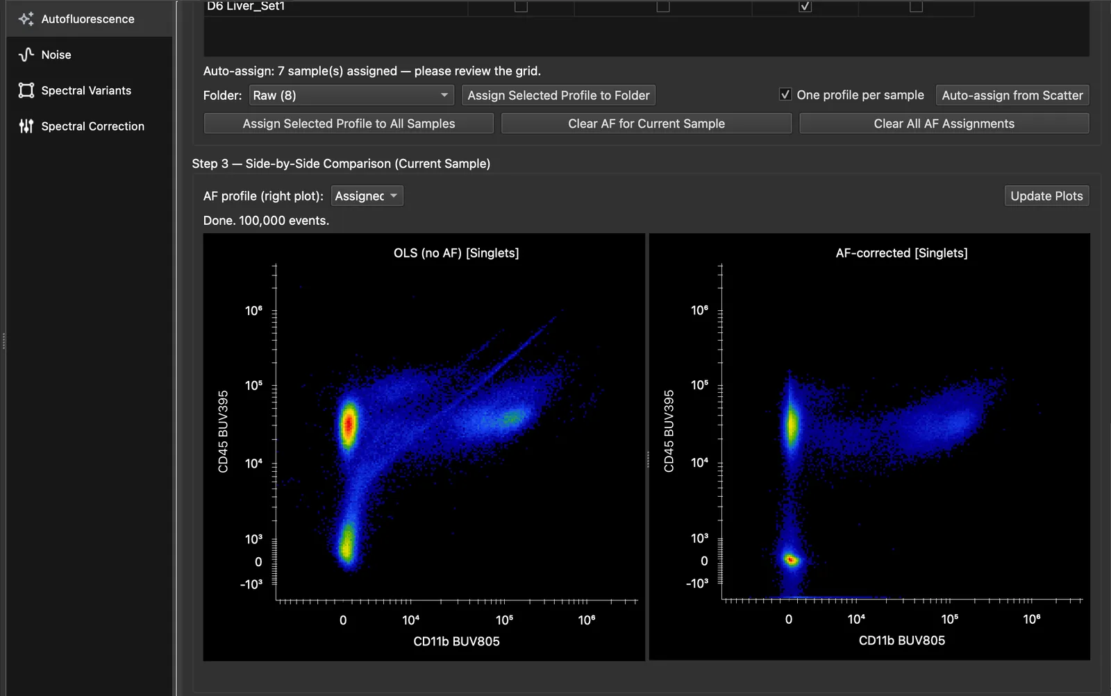
Step 3 for an unstained sample: CD45 BUV395 against CD11b BUV805, a long diagonal autofluorescence streak without AF extraction and a compact population at zero with per-cell AF — Step 3 for an unstained sample. Without AF extraction (left), autofluorescence reads as a diagonal streak into CD45 BUV395 and CD11b BUV805; with per-cell AF (right), the cells sit at zero.

Step 3 for a stained sample: CD45 BUV395 against CD11b BUV805, without AF extraction and with per-cell AF — Step 3 for a stained sample. Per-cell AF removes the diagonal streak and the false CD45 and CD11b signal, leaving the real populations.

What good looks like: negatives sit at zero and are compact, and the diagonal spikes and skews of the left plot are gone. If a population still sits off zero, its autofluorescence may be missing from the unstained sample. Extract a profile from an unstained sample that contains those cells, and assign it too.

What changes in your data

Every sample with an assigned profile is now unmixed with per-cell AF everywhere it is used: plots, Simple Stats, exports and the analysis plugins. Two channels are added to the unmixed data, and you can plot and gate on both:

AF Abundance: how much autofluorescence was removed from each cell.
AF Index: which AF spectrum was chosen for each cell. In the AutoSpectral study, the AF Index tracked scatter, cell type and imaging parameters.

Samples without a profile are unmixed by ordinary least squares as before.

Next, optionally, the noise model or the spectral variants.

Autofluorescence

Step 1: extract an AF profile from each unstained sample

Step 2: assign profiles to samples

Auto-assign from scatter

Step 3: compare

What changes in your data

Further reading