Cytkit | Honeychrome
 Honeychrome
- Overview and Installation
- Acquire Data
- Spectral Analysis
- AutoSpectral in Honeychrome
- Conventional Analysis
- Manipulate Plots and Gates
- Reports, Exports & Sample Comparison
- Programming and Plugins
AutoSpectral in Honeychrome
AutoSpectral is an optimised unmixing workflow.
Originally written in R, AutoSpectral is a set of tools to enhance spectral analysis by providing you with the best possible spectral signatures of your spectral controls, optimising the removal of autofluorescence, and providing reproducible mixing. See the Colibri Cytometry blog and the AutoSpectral Github repository for more information on AutoSpectral.
Honeychrome now provides the following two major components of AutoSpectral natively as steps in the spectral process:
- AutoSpectral Cleaning (optimisation of control profiles)
- AutoSpectral AF (per-cell autofluorescence extraction)
AutoSpectral Cleaning clears up artifacts due to poor single stain control profiles, for example hypernegative events, skewed data and diagonal correlations, by carrying out saturation exclusion, brightest-event selection, scatter matching and noise removal on the control profiles.
AutoSpectral AF clears up artifacts due to variable autofluorescence, for example negative spreading, by pairing every event with its best matched autofluorescence spectrum.
See related articles on Colibri Cytometry: AutoSpectral Cleaning and AutoSpectral AF
This guide assumes you have already installed Honeychrome using the executable installers (Windows/Mac/Linux) or Python (cross-platform), that you have a set of FCS files to import, and that you are already familiar with the basic spectral unmixing process. If not, please go to Spectral Analysis first.
We will be continuing use of AutoSpectral Full Workflow Example (a 9-colour panel from the 5-laser Cytek Aurora from the AutoSpectral Full Workflow Example as set up in the tutorial Spectral Analysis.
How to perform AutoSpectral Cleaning (optimisation of control profiles)
Show the AutoSpectral Cleaning process and click “Clean Controls”
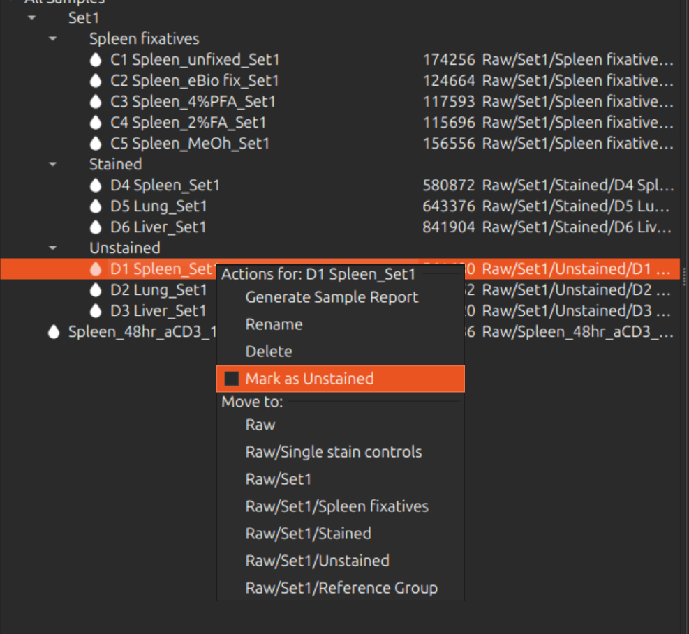
First make sure that you have at least one unstained control (i.e. with “unstained” in the name) in the single stain controls folder. Preferably, you should have additional unstained controls if you are dealing with cell types that have variable autofluorescence. You can mark any additional samples as unstained in the Sample Browser (left pane) by right clicking them and checking “Mark as Unstained”. Unstained samples are marked in the sample browser with a blue droplet icon.
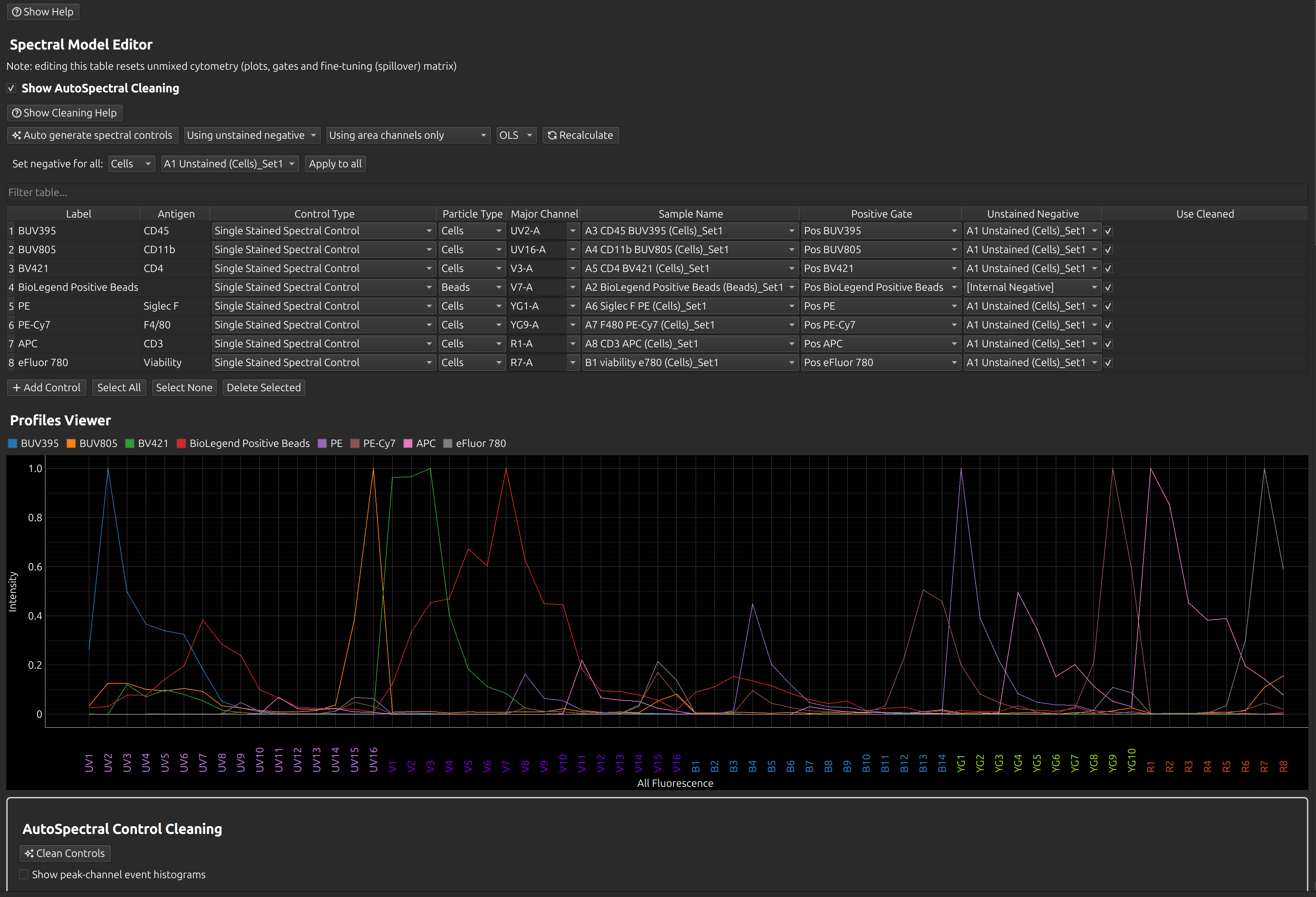
Now in the Spectral Process tab, generate your spectral controls (e.g. with the Autogenerate Spectral Controls button, see Spectral Analysis). Make sure you select “Using unstained negative” instead of “Using internal negatives”.
Click “Show AutoSpectral Cleaning”, which brings up the AutoSpectral control cleaning box and a workflow help guide.
Two new columns are shown in the spectral controls table: “Use cleaned” and “Exclude Noise”. The cleaned profiles are applied when you run Clean Controls. The noise removal is not checked by default, as it is not necessary for controls with low autofluorescence: run it first and see the results. Then consider applying noise removal to controls with high autofluorescence and re-running.
You may now click “Clean Controls”. The AutoSpectal cleaning pipeline will automatically proceed. Each control will be processed for:
- Saturation exclusion
- Brightest-event selection
- Scatter matching (selection of the best-matching negative cells)
- Noise removal (subtraction of matching autofluorescence per control event)
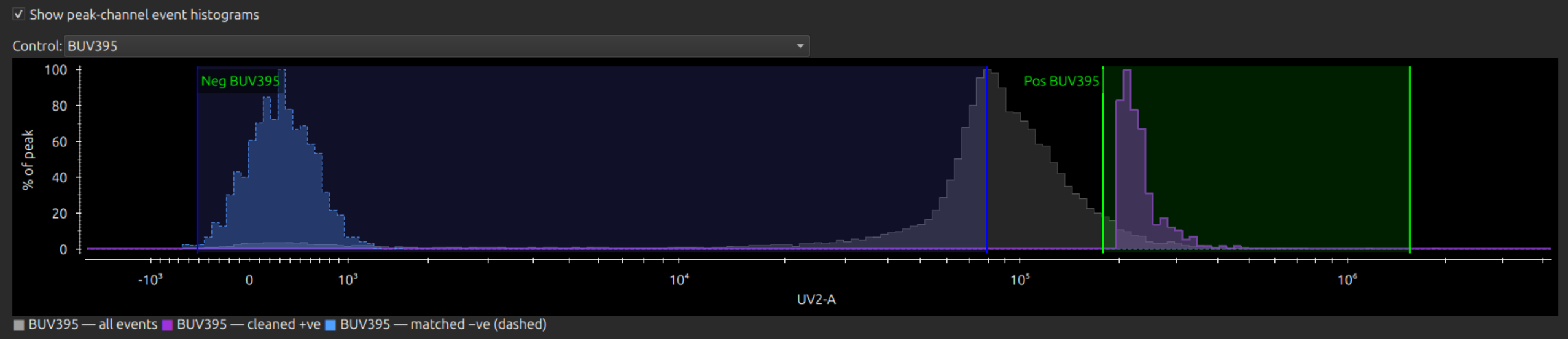
Show peak channel event histograms
There is now a checkbox below the spectral model table, “Show peak channel event histograms”. Enable this and click on a line of the spectral model table to see the events selected for both positive and negative controls after control cleaning, against all events in that sample.
You can adjust the gating here before re-running control cleaning.
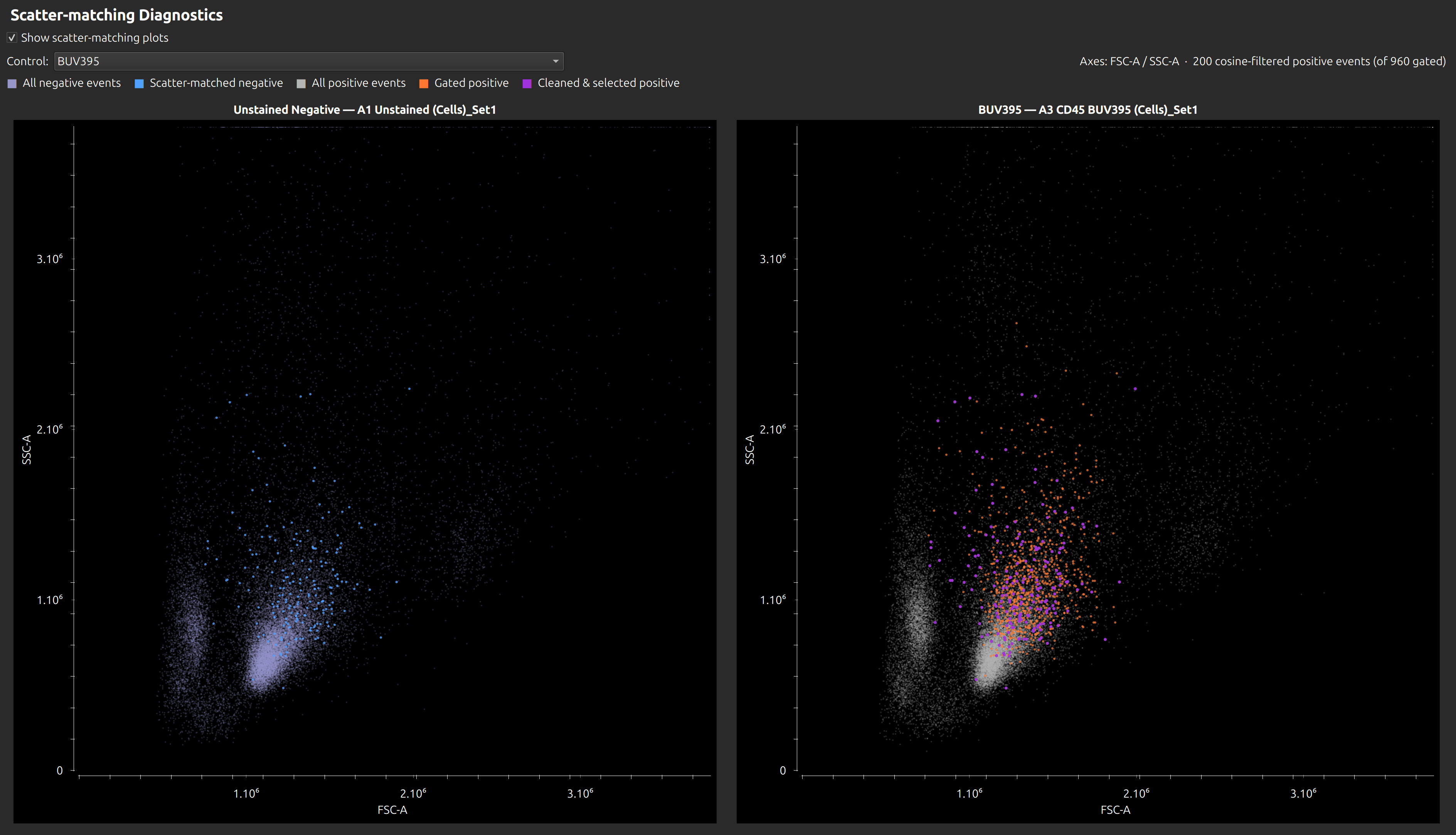
Scatter-matching Diagnostics
A further checkbox “Show scatter-matching plots” is shown. These show the unstained cells that best match the positive cells on the morphology plot, and are therefore the best choice to use for negatives of that profile.
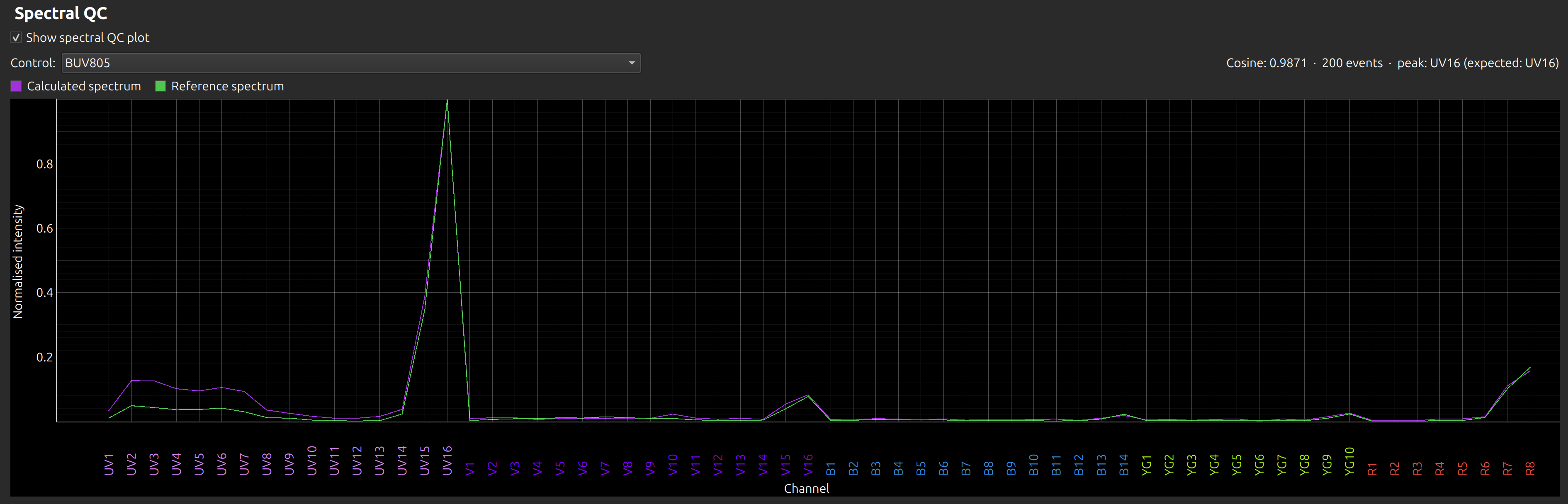
Spectral QC
A further checkbox “Spectral QC” is shown, which .
How to perform AutoSpectral AF (per-cell autofluorescence extraction)
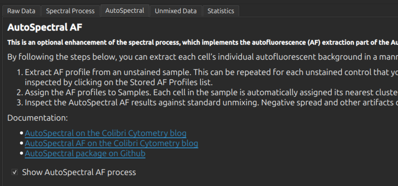
Show the AutoSpectral AF process
Go to the AutoSpectral tab and check the box “Show AutoSpectral AF process”
Extract AF profile from an unstained sample
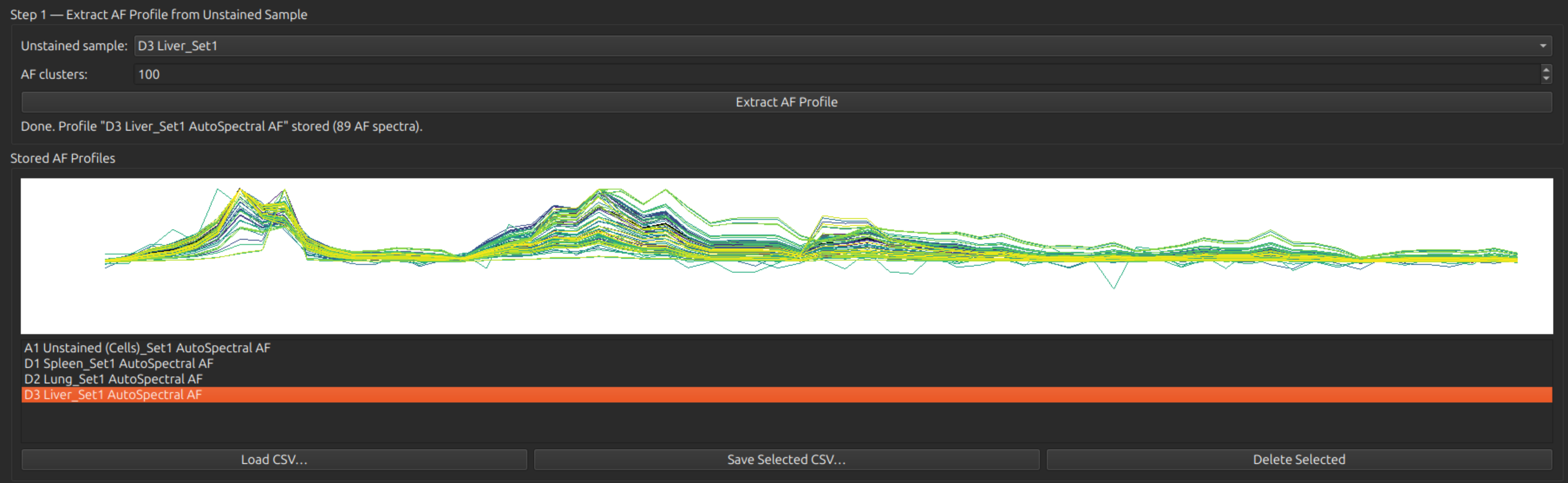
Under Step 1, select your (first) unstained sample, and press the button Extract AF Profile. (Default number of clusters: 200.) You should see a set of spectra of clusters below. This step should be repeated for each unstained control that you have available, generating multiple AF profiles. After extraction, the clusters can be inspected by clicking on the Stored AF Profiles list.
Assign the AF profiles to samples
Under Step 2, select the AF profiles to apply to each sample. Multiple controls (columns) can be selected for each sample (row). Each cell in the sample will be automatically assigned its nearest cluster from of the selected controls for a more accurate AF subtraction.

Inspect the AutoSpectral AF results against standard unmixing
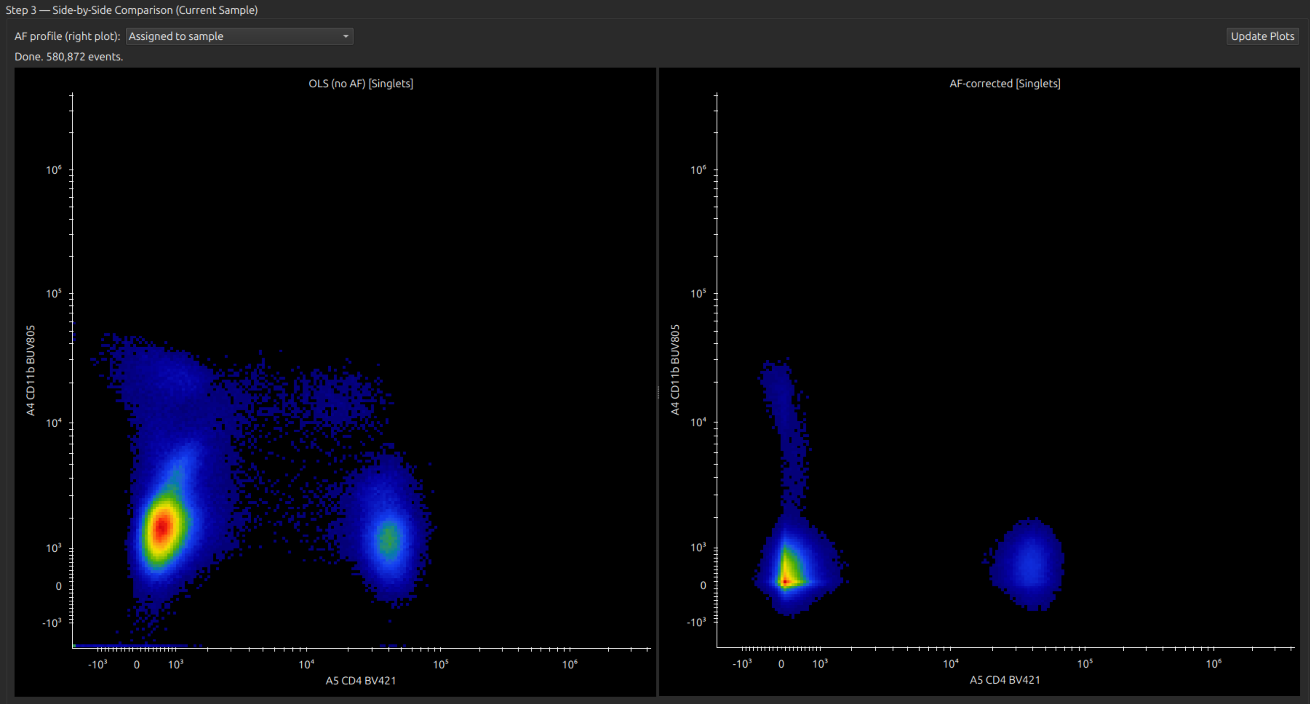
Under Step 3, select a sample (from the sample browser, left pane), and select channels and a source gate on the side-by-side plots.
Negative spread and other artifacts caused by inhomogeneous autofluorescence should be much improved.
This workflow recalculates all unmixed data for analysis in the Unmixed Data / Statistics tabs, and is applied whenever an assigned sample is loaded in the sample browser.